
Motivation
Modern reasoning systems don’t have to rely on the first answer generated by an LLM. In fact, it’s now understood that effort expended after the model has been trained can be more effective than more training effort or increased parameters (e.g., Snell et al. 2024; Wu et al. 2024).
A common way to use this test-time compute is to sample many candidate outputs from the model, and to judge them in some fashion using a verifier[1]. The resulting system separates three tasks: the generator (LLM) proposes outputs, the verifier scores them, and the selector uses the scores to decide which candidate is surfaced to the user. An early example of this was given by Cobbe et al. (2021) in the context of mathematical reasoning. Provided the model has some non-zero probability of generating the right answer, and the verifier can identify it, the benefit is clear. We simply keep generating until our oracle verifier (which identifies correctness without error) is satisfied or, for a fixed budget, sample \(N\) candidates, rank them by verifier score and return the highest-scoring one. The latter procedure is known as Best-of-\(N\) selection; we’ll return to it in detail in a later post in this series.
Under these assumptions, scaling test-time compute can only ever help us, at some computational cost. Unfortunately, there is no guarantee the model can generate a correct output and oracle verifiers don’t exist for most relevant tasks, so in practice the success of the approach rests heavily on the quality of generation and of the verifier model.
If you’re interested in how language models are encouraged to reason well through training, take a look at the review post Training for reasoning: a short note.
Reasoning strategies at test time
Snell et al. (2024) frames test-time scaling, also called inference-time scaling, as
modifying the model’s predicted distribution adaptively at test-time, conditioned on a given prompt.
What do they mean by this? Let \(\pi\) denote the current generator[2]. For a problem presented through a prompt \(x\), the generator defines a proposal distribution \(\pi(\cdot \mid x)\) over its outputs[3]. For definiteness, we use \(\pi(\cdot \mid x)\) to denote the complete sampling law, including stopping, maximum length, temperature and any top-k or top-p truncation. It isn’t determined by the network weights alone.
Snell et al. describe two ways in which test-time compute can be used to modify the model’s predicted distribution: input and output level.
At the input level
Input-level methods change the information presented to the generator. A system might ask the model to critique an initial attempt, revise it (Madaan et al. 2023), or explore a problem over several turns (Shinn et al. 2023) before constructing a new prompt \(\widetilde{x}\). The final output is then drawn from
\[ \widetilde{Y}\sim\pi(\cdot\mid\widetilde{x}). \]
Through critique and other non-deterministic methods, \(\widetilde{x}\) may itself be the realized result of a stochastic adaptive procedure; the displayed law is then conditional on that realized prompt. The aim is that \(\widetilde{Y}\) is on average a better output for the prompt \(x\) than the base output \(Y\sim\pi(\,\cdot\mid x)\).
At the output level
Output-level strategies typically sample several candidate outputs and compare or combine them in some way (Cobbe et al. 2021). This is where we’ll focus our efforts in this series. Setting up some notation, suppose we sample \(N\) candidate outputs \(Y_1,\ldots,Y_N\) from \(\pi(\,\cdot\mid x)\), and abbreviate this as \(Y_{1:N}:=(Y_1,\ldots,Y_N)\); we’ll call this the candidate pool.
A selector is a rule that takes the candidate pool as input and returns a single output:
\[ Y^\star = \operatorname{Sel}_N\!\left(x;Y_{1:N}\right). \]
Any scoring or checking is included in this rule. We’ll assume the selector is deterministic given \(x\) and \(Y_{1:N}\) to keep the notation light[4]. This is quite a generic setup, and the selector as written could use exact correctness checks, consensus voting, or a learned verifier to rank the candidates. The final selected output has its own distribution, which we write as
\[ Y^\star \sim q_N(\,\cdot\mid x) \] where we’ve left the dependence on the selector implicit. Equivalently, for each output \(y \in \mathcal{Y}\), \[ q_N(y \mid x) = \underset{Y_{1:N}}{\Pr}\!\left(\operatorname{Sel}_N(x;Y_{1:N})=y\right), \] which we call the served-output distribution.
Additional assumptions
The setup so far is general, and captures almost every approach. We’ll now make a number of assumptions that we’ll carry through the rest of the series. In making these assumptions, we restrict our attention to a sizable class of popular test-time methods and gain the ability to make mathematical progress in analyzing them.
\[ Y_1,\ldots,Y_N \stackrel{\mathrm{iid}}{\sim} \pi(\,\cdot\mid x), \qquad N \text{ fixed in advance}. \]
The candidates are iid from a fixed generator, and \(N\) is fixed in advance and independent of the prompt or the candidates themselves.
Same prompt and generator for every draw. Methods like Self-Refine (Madaan et al. 2023) and Reflexion (Shinn et al. 2023), as their names suggest, generate later draws from a prompt derived from earlier draws.
Independent draws. Some methods don’t generate outputs independently, but run them forward for some number of steps and then decide which to continue, or how to weight them, and so on. Some examples include Tree of Thoughts (Yao et al. 2023), PRM-guided beam search (Snell et al. 2024), and sequential Monte Carlo methods like Rollout Roulette (Puri et al. 2025) and twisted SMC (Zhao et al. 2024) that we’ll discuss in more detail in a later post in this series. Worth noting – outputs generated in this way are dependent and generally no longer follow the original proposal distribution \(\pi\).
\(N\) fixed in advance. Rather than fixing the budget in advance, it’s possible to allocate compute dynamically, perhaps by problem difficulty (Snell et al. (2024) again) or sampling until a condition is met (Adaptive-Consistency (Aggarwal et al. 2023)).
Choosing \(N\) from the prompt before sampling preserves our per-prompt coverage formula, whereas stopping based on generated candidates generally does not; we use a common \(N\) across prompts for the population bounds below.
\[ Y^\star=\operatorname{Sel}_N\!\left(x;Y_{1:N}\right)\in\{Y_1,\ldots,Y_N\}. \]
The selector returns one sampled candidate unchanged; it does not combine, modify or reassemble candidates.
LLM-Blender (Jiang et al. 2023) and Mixture-of-Agents (Wang et al. 2024) are examples of fusion, where candidates are (optionally) ranked and then merged in some fashion.
If you’re interested in approaches outside of the assumptions taken here, Zhang et al. (2025) give a broad review of test-time scaling methods.
Under the selector assumption, for \(N=1\), the proposal and served-output distributions coincide. For higher \(N\), they generally don’t. Note, too, that \(\operatorname{supp}(q_N)\subseteq \operatorname{supp}(\pi)\). The end-to-end setup is illustrated in Fig. 1.
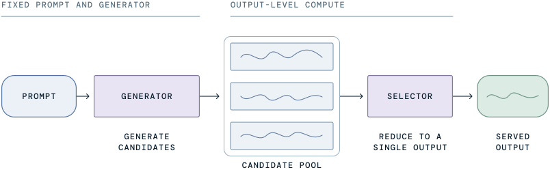
This setup raises many questions: What information can a selector use? How quickly does candidate coverage (the probability that at least one candidate is correct) grow with \(N\)? How much of that candidate coverage does the selector convert into correct served outputs? As \(N\) increases, which regions of the proposal distribution does \(q_N\) upweight, particularly where the selector is wrong?
We hold the generator fixed throughout, and the prompt fixed except when averaging over a population of problems. We vary the candidate budget and selector. Our central interest is the resulting served-output distribution \(q_N(\cdot \mid x)\).
Test-time search
The previous section described how applying a selector \(\mathrm{Sel}_N\) with a candidate budget \(N\) to a fixed generator \(\pi\) induces a served-output distribution \(q_N\). What we really care about is how these choices affect the probability of the system returning a correct output to the user.
Repeated sampling
Let’s first gain some intuition by trying to pin down mathematically why we should be at all optimistic about sampling more than once from the model. For now, we put selectors to one side and take a step back. Suppose we’re generating outputs from a generator \(\pi\), conditional on a prompt \(x\).
Let \(c(x, y) \in \{0, 1\}\) indicate whether output \(y\) gives a correct final answer for \(x\).
This is the last of the major standing assumptions we make throughout this series, and it comes in three parts.
Correctness is binary. The extracted final answer is either correct, or it isn’t; there’s no grading or partial credit.
Correctness is a fixed function of the prompt and the output. First, it’s a function in the sense that it’s a fixed, deterministic map. We also take ‘truth’ here to be an exogenous property; it isn’t defined by the model, evaluator etc.
Correctness depends on the output only through its extracted final answer. We’ll call an output correct when its extracted final answer is correct. This is different from requiring the reasoning trace itself to be valid, since a model can arrive at the right answer for the wrong reasons. Equally, sound reasoning can be followed by an incorrect answer. We return to this distinction when discussing outcome and process verifiers.
These assumptions concern correctness itself; a selector may still use graded scores or assess intermediate reasoning.
For any conditional output law \(\mu(\cdot\mid x)\), define its per-prompt accuracy as
\[ \begin{aligned} a_\mu(x) &\triangleq \underset{Y\sim\mu(\cdot\mid x)}{\mathbb E}\!\left[c(x,Y)\right] \\[0.8em] &= \underset{Y\sim\mu(\cdot\mid x)}{\Pr}\!\left(c(x,Y)=1\right). \end{aligned} \tag{1}\]
For the generator, \(a_\pi(x)\) is therefore its single-sample accuracy for prompt \(x\): the probability of an output having a correct final answer. Suppose that \(a_\pi(x)>0\). Let’s now draw our candidate pool:
\[ Y_1,\ldots,Y_N \stackrel{\mathrm{iid}}{\sim} \pi(\,\cdot\mid x). \tag{2}\]
Since we’ve drawn \(N\) iid samples, the probability that none gives the correct answer is
\[ (1-a_\pi(x))^N \xrightarrow[N \to \infty]{} 0, \]
and therefore repeated sampling eventually produces a correct answer with probability one. It may sound too good to be true, and in reality it is. By thinking about where this equation breaks down, we can uncover some of the shortcomings of this approach.
Firstly, it relies on some correct output having positive probability under the proposal distribution. In other words, we need \(a_\pi(x)>0\). This is certainly not guaranteed, but can be influenced by improvements to training or, at test time, input-level strategies. Yet for a new problem we generally don’t know \(a_\pi(x)\) exactly or have a reliable lower bound for it.
Even if we knew that \(a_\pi(x)>0\), the probability may be far too small to practically exploit. Without truncation and with positive token probabilities, every finite complete output has positive probability. In other words, unless the output is truncated (by setting a length cap, or using top-\(k\) or top-\(p\)), the issue you face is that the correct output may be very unlikely to be sampled.
While on the face of it these drawbacks seem to be bad news, we nonetheless see in practice that using multiple samples from the model can substantially increase average candidate coverage. An example from Cobbe et al. (2021) makes our point: early in fine-tuning, their 6B generator solved ~19% of GSM8K problems using (deterministic) greedy decoding, while 100 sampled outputs contained a correct answer for ~84%[5]. This makes intuitive sense. The probability of sampling a correct answer varies across problems. For a subset, the greedy decoding output contains a correct final answer. The remaining questions are, in principle, where the biggest gains will be made from repeated random sampling. The probability of generating at least one correct answer for these problems increases monotonically with the budget \(N\) whenever the probability of a correct output is positive. On this point, Brown et al. (2024) found, across multiple models and tasks, that average candidate coverage grows roughly log-linearly with \(N\) over four orders of magnitude. This line of thinking also tells us why we don’t expect repeated sampling to take us all the way to 100% average candidate coverage. For any given model, there will exist some problems requiring reasoning that is outside of the support of the model, or vanishingly unlikely, in order to be correctly solved. Those problems will never be solved by the model with any practical budget.
We’re ready to define candidate coverage, that is, the probability of the candidate pool containing at least one correct candidate. Continuing from the setup of Eq. 2, define
\[ \operatorname{Cover}_N(x) \triangleq \underset{Y_{1:N}\sim\pi(\cdot\mid x)^{\otimes N}}{\Pr}\!\left(\exists i\leq N:c(x,Y_i)=1\right). \]
Note that candidate coverage is not the probability that the system returns a correct output; it says only whether a correct candidate is available to be selected.
EXAMPLE Candidate coverage from repeated sampling
Under our sampling assumption, candidate coverage is
\[ \operatorname{Cover}_N(x) = 1 -(1-a_\pi(x))^N. \]
Notice that this increases monotonically in \(N\). To obtain candidate coverage at least \(1-\delta\), for \(0 < a_\pi(x) < 1\) and \(0 < \delta < 1\), rearranging this equation shows
\[ N_{\min}=\left\lceil\frac{\log\delta}{\log(1-a_\pi(x))}\right\rceil. \]
When \(a_\pi(x)\) is small, \(\log(1-a_\pi(x))\approx-a_\pi(x)\), so
\[ N_{\min}\approx\frac{\log(1/\delta)}{a_\pi(x)}. \]
Thus the required sampling budget grows approximately inversely with single-sample accuracy and logarithmically with the desired inverse failure probability \(1/\delta\). Naturally, if \(a_\pi(x) = 1\), only one sample is needed, and if \(a_\pi(x) = 0\) then no amount of sampling can give the right answer.
If each draw from the model produces the correct answer with 1% probability, say, and we seek 95% candidate coverage, the exact expression gives \(N_{\min}=299\) (while the approximation gives about 300).
Across a population of problems, with prompts \(X\sim\mathcal D\), average candidate coverage is simply the familiar metric \(\operatorname{pass@N}=\mathbb E_{X\sim\mathcal D}[\operatorname{Cover}_N(X)]\) (Chen et al. 2021).
You may be asking – can we predict the gains from repeated sampling if we know a model’s average single-sample accuracy? In other words, if we know a model’s \(\operatorname{pass@1}\) can we predict its \(\operatorname{pass@N}\)? We can only give bounds, but in order to understand the relationship precisely we’d need to know how the probability of success varies across problems. It’s instructive to think about why.
Imagine two generators, \(\pi_1\) and \(\pi_2\), tested on the same benchmark and found to have an identical average single-sample accuracy, that is, an identical \(\operatorname{pass@1}\). Suppose that
- \(\pi_1\) solves every problem with probability 0.5 on each draw.
- \(\pi_2\) is constructed so that it gets half of the benchmark problems correct every time, and half wrong every time.
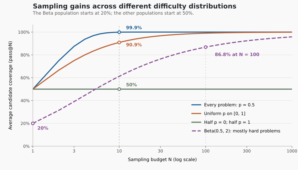
Both have \(\operatorname{pass@1} = 0.5\), but the gains they each make from repeated sampling are completely different. By construction, \(\pi_2\) stands to gain nothing at all, and its \(\operatorname{pass@1}\) and \(\operatorname{pass@N}\) are equal. In contrast, \(\pi_1\) benefits from repeated sampling for any prompt \(x\), since for this model \(\operatorname{Cover}_N(x) = 1 -(\frac{1}{2})^N\), which is approximately 99.9% for \(N=10\).
In general, under the sampling assumptions we’ve made in this post, we know
\[ \operatorname{pass@N} =\mathbb E_{X\sim\mathcal D}\!\left[1-(1-a_\pi(X))^N\right] \;\le\; 1-\bigl(1-\mathbb E[a_\pi(X)]\bigr)^N. \] The first equality is a definition along with our assumptions. The inequality that follows is an application of Jensen’s inequality, since for \(N>1\), the function \(p\mapsto 1-(1-p)^N\) is strictly concave. Note that we also have a lower bound, since \(\operatorname{pass@N} \geq \operatorname{pass@1}\). Finally, letting \(m = \operatorname{pass@1}\), we get
\[ m \leq \operatorname{pass@N} \leq 1-\bigl(1-m\bigr)^N. \]
These bounds are tight: our generators \(\pi_1\) and \(\pi_2\) attain the upper and lower bounds respectively.
The statement tells us that if we have access to the benchmark average success probability \(\mathbb E[a_\pi(X)]\), and use this in place of the per-problem success probability, we obtain an upper bound on \(\operatorname{pass@N}\), attained when the probability of success is the same across all benchmark problems.
Average single-sample accuracy therefore bounds average candidate coverage over a problem population, but doesn’t determine it. For that, we’d need to know how the probability of success varies across problems in the benchmark.
If success probabilities across a hypothetical population are uniformly distributed on \([0,1]\), average candidate coverage is \(N/(N+1)\). More generally, for a \(\operatorname{Beta}(\alpha,\beta)\) distribution, with \(\alpha,\beta>0\), its shortfall from one decays like \(N^{-\alpha}\) for large \(N\). These examples show how the amount of probability mass near zero success probability controls the rate at which coverage improves (Fig. 2).
TECHNICAL NOTE How difficulty shapes coverage
Write \(p=a_\pi(X)\) for the single-sample accuracy of a randomly drawn problem. Under our sampling assumption, the average probability that no candidate is correct is \(\mathbb E[(1-p)^N]\).
If \(p\) is uniformly distributed on \([0,1]\),
\[ \mathbb E[(1-p)^N]=\int_0^1(1-p)^N\,\mathrm dp=\frac{1}{N+1}. \]
Consequently, average candidate coverage is \(N/(N+1)\). Failure to generate a correct candidate decays exponentially in \(N\) for each fixed problem with \(0<p<1\), but like \(1/N\) after averaging over this population. Under the uniform assumption, a fraction \(1/N\) of problems have success probability at most \(1/N\). Each has failure probability at least \((1-1/N)^N\) after \(N\) draws, which tends to \(e^{-1}\approx37\%\) as \(N\) grows.
More generally, suppose \(p\sim\operatorname{Beta}(\alpha,\beta)\), with \(\alpha,\beta>0\). Its density is \(p^{\alpha-1}(1-p)^{\beta-1}/B(\alpha,\beta)\), where \(B\) is the beta function. Then
\[ \begin{aligned} 1-\operatorname{pass@N} &=\frac{1}{B(\alpha,\beta)}\int_0^1p^{\alpha-1}(1-p)^{\beta+N-1}\,\mathrm dp\\[0.5em] &=\frac{B(\alpha,\beta+N)}{B(\alpha,\beta)}\\[0.5em] &=\frac{\Gamma(\alpha+\beta)}{\Gamma(\beta)} \frac{\Gamma(\beta+N)}{\Gamma(\alpha+\beta+N)}\\[0.5em] &\sim\frac{\Gamma(\alpha+\beta)}{\Gamma(\beta)}N^{-\alpha} \qquad (N\to\infty), \end{aligned} \]
where \(\Gamma\) is the gamma function; the last step uses \(\Gamma(N+b)/\Gamma(N+a+b)\sim N^{-a}\). The uniform case is \(\alpha=\beta=1\). The exponent \(\alpha\) describes the density near zero success probability: smaller \(\alpha\) gives slower decay. These are hypothetical population distributions, not the exact empirical distribution of a finite benchmark.
Next we’ll discuss the simplest kind of selector, where correctness can be checked directly.
Exact checks
In some verifiable domains, correctness can be checked exactly. Recall that \(q_N(\cdot\mid x)\) is the distribution of the selected output \(Y^\star\). Applying Eq. 1 to this distribution gives the served accuracy for prompt \(x\),
\[ a_{q_N}(x) =\underset{Y^\star\sim q_N(\cdot\mid x)}{\Pr}\!\left(c(x,Y^\star)=1\right). \]
Suppose a checker accepts precisely those candidates for which \(c(x,y)=1\), and the selector returns an accepted candidate whenever one exists. The system then serves a correct output exactly when the candidate pool contains one, so
\[ a_{q_N}(x)=\operatorname{Cover}_N(x). \]
For a fixed generator and candidate budget, this is as good as it gets.
It’s worth mentioning a practical wrinkle to the idea of verifiable domains. Even domains that at face value seem verifiable can turn out not to be, as a result of practical or cost constraints. Code, for example, can practically be checked up to a finite suite of tests (Li et al. 2022). Passing such tests doesn’t prove the logic of the code is valid, nor does the validity of checked behavior necessarily extend to untested behaviors.
Beyond exact checks
Exact checking is possible in only a few domains. Outside of those, we need to rely on verification with inherent flaws. In those cases, even if the candidate pool contains a correct candidate, we aren’t guaranteed to pick it. The served accuracy, defined above, can then be written as a sum over all possible outputs,
\[ a_{q_N}(x) =\sum_{y\in\mathcal Y}q_N(y\mid x)c(x,y). \]
Under the standing selector assumption, a served output can be correct only if the pool contained a correct candidate. It follows that
\[ a_{q_N}(x)\leq\operatorname{Cover}_N(x), \]
and the gap has a direct interpretation:
\[ \operatorname{Cover}_N(x)-a_{q_N}(x) =\Pr\!\left(\exists i:c(x,Y_i)=1,\;c(x,Y^\star)=0\right). \]
The bound also holds for dependent candidates, with candidate coverage computed under their joint distribution.
TECHNICAL NOTECANDIDATE COVERAGE Why candidate coverage upper-bounds served accuracy
Another way to see this, which provides some insight, is the following. For a fixed prompt \(x\) and candidates \(Y_1,\ldots,Y_N\stackrel{\mathrm{iid}}{\sim}\pi(\,\cdot\mid x)\) define the events
\[ \begin{aligned} A&=\{\exists i\leq N:c(x,Y_i)=1\}, \quad \mathrm{and} \\[1em] B&=\{c(x,\operatorname{Sel}_N\!\left(x;Y_{1:N}\right))=1\}. \end{aligned} \]
All probabilities in this note are taken over candidate generation, with \(x\) held fixed. For the randomized extension described above, selector randomness is included too. Since the selector must return one of the candidates, \(B\subseteq A\). It also follows that \(\Pr(A\setminus B)=\Pr(A)-\Pr(B)\). Finally, by definition, \(\Pr(A)=\operatorname{Cover}_N(x)\).
Consequently,
\[ \operatorname{Cover}_N(x)-a_{q_N}(x) =\Pr(A\setminus B) =\Pr\!\left(\exists i:c(x,Y_i)=1,\;c(x,Y^\star)=0\right). \]
We’ll use the term loss for two useful failure probabilities. Selection loss is the probability that a correct candidate was available but the selector served an incorrect one. Generation loss is the probability that generation failed to produce any correct candidate at the chosen budget. The served error probability decomposes as
\[ 1-a_{q_N}(x) =\underbrace{1-\operatorname{Cover}_N(x)}_{\vphantom{\Huge A}\text{generation loss}} +\underbrace{\operatorname{Cover}_N(x)-a_{q_N}(x)}_{\vphantom{\Huge A}\text{selection loss}}. \]
The two losses describe different problems. More or better sampling can reduce generation loss by making a correct candidate more likely to appear. Better judgment can reduce selection loss by recognizing a correct candidate that’s already present, but it can’t create one.
Summary
We’ve established exactly how repeated sampling improves candidate coverage, making a correct candidate more likely to appear. How quickly average candidate coverage improves depends on the distribution of problem difficulty within the problem set in question. Using the average single-sample accuracy can be misleading as it provides only bounds, and doesn’t uniquely determine the improvement.
For the system to return a correct output requires success not only in sampling, but in selection, too. We saw a decomposition of the served error probability that splits into generation and selection loss. We know we can reduce generation loss using larger \(N\), but it isn’t exactly clear what the effect of larger \(N\) is on selection. We’ll turn our attention to this in future posts.
Next time: consensus voting as a selection mechanism. When does it work, when does it fail, and why?
I’ll use the term verifier for any mechanism that scores candidate outputs. When the scorer is learned, the literature often calls it a reward model, and we’ll see a few examples later that use this terminology.
Here, the generator is the LLM together with its decoding settings. ‘Policy’ is the corresponding reinforcement learning term.
In case it feels a little hand-wavy, there are ways to make this rigorous. Let \(\mathcal{V}\) denote the model’s token vocabulary. A complete output is a finite token string \(y=(y_1,\ldots,y_T)\), with stochastic length \(T\), so the space of possible outputs is \[ \mathcal{Y}=\bigcup_{\ell\geq 0}\mathcal{V}^{\ell}, \] commonly written \(\mathcal{V}^{\ast}\) using the Kleene star. Generation stops at the first end-of-sequence (EOS) token, which is retained, or at the maximum length. Autoregressively, the probability of such a complete output is \[ \pi(y\mid x) = \prod_{t=1}^{T} \pi\!\left(y_t\mid x,y_{<t}\right), \] where \(y_{<t}=(y_1,\ldots,y_{t-1})\), and the token probabilities include temperature scaling and any top-\(k\) or top-\(p\) truncation. All other strings have probability zero.
If the selector includes some stochastic component(s), we can simply include its randomness as an independent random variable in the joint distribution and marginalize it out. Nothing changes in the subsequent arguments because, whatever the value of the random variable, the selector always returns one of the candidates.
Note, this isn’t quite the \(N=1\) and \(N=100\) endpoints of the same experiment. Greedy decoding is different from taking one stochastic draw from the sampling law used to form the candidate pool. Here, greedy decoding used \(T=0\), while the 100 samples used \(T=0.7\).